


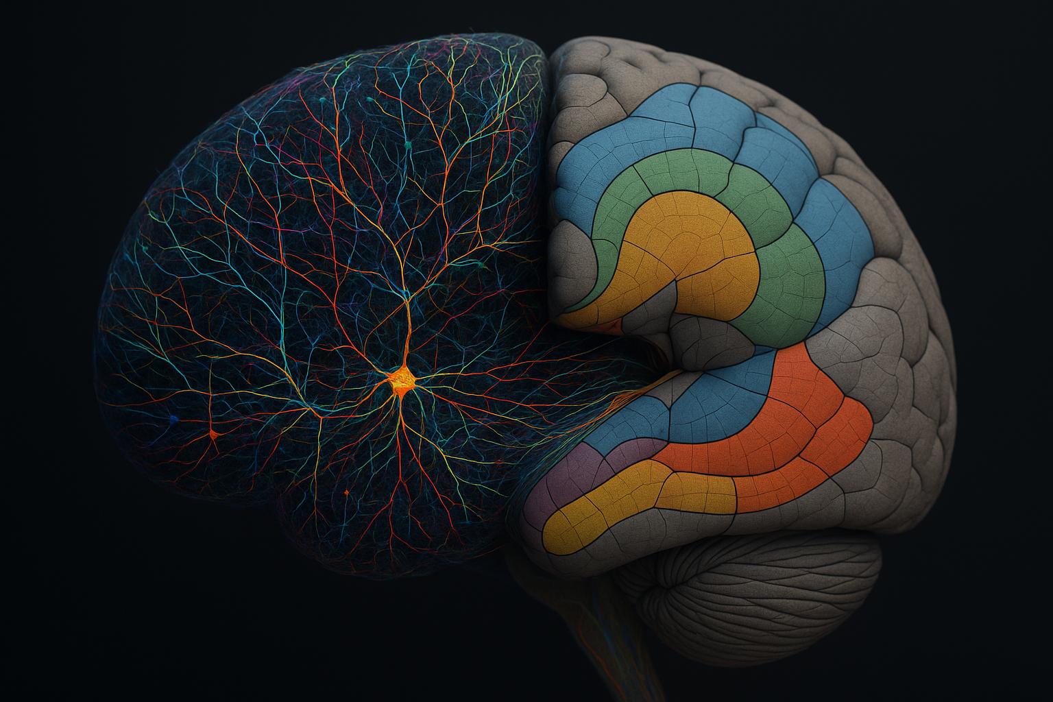
Shoppers of cutting-edge neuroscience tools, rejoice: researchers have unveiled a suite of mapping technologies that let labs align full 3D brain atlases to partial, high‑resolution spatial transcriptomics data, cutting the pain of missing slices, gargantuan file sizes and feature overload , and making atlas-to-cell maps more robust, practical and faster to run.
- Censoring works: a spatial support function masks atlas regions not sampled, so partial serial sections (or hemi‑brains) align cleanly to whole‑brain atlases. Smarter focus means fewer false deformations.
- Scale‑space particle resampling: the team builds optimal, multi‑scale particle approximations (50–200 μm) that keep spatial detail while slashing computational load; these move slightly to hug tissue curves and feel more “natural” than grid resampling.
- Mutual‑information feature selection: picking the most spatially informative genes keeps inter‑region contrasts high while reducing feature noise; 20 high‑MI genes from a 500‑gene MERFISH set captured atlas boundaries well.
- Cross‑modality via varifolds: a unified image‑varifold representation ties physical location and functional features (genes, cell types, regions) into one norm that beats naive Euclidean comparisons.
- Practical performance: the pipeline maps BARseq, MERFISH and cycleHCR datasets to Allen CCFv3 and EMAP atlases with accuracy comparable or superior to manual slice‑by‑slice methods, while keeping runtimes reasonable on GPUs.
Why this mapping toolbox matters right now
Spatial transcriptomics is exploding, but experiments often sample only parts of a brain or embryo because of cost and technical limits. That mismatch makes it painful to fit partial, high‑resolution reads into tissue‑scale atlases. This work introduces three modular fixes , censoring, optimized particle resampling, and mutual‑information feature selection , that slot into a varifold‑based diffeomorphic mapping pipeline (xIV‑LDDMM) and handle partial volumes, varying resolution and cross‑modality differences in one coherent framework. The result is alignment that feels less brittle and more honest to the messy realities of real experiments.
How censoring tames partial and uneven data capture
Think of censoring as telling the atlas “only try to match where you actually have data.” The authors add a smoothly varying support weight into the atlas representation that goes from 1 inside the measured tissue to 0 outside it. That avoids forcing the atlas to invent matches in unmeasured poles or across dropped slices, and it keeps the diffeomorphic transform from stretching the atlas to cover missing tissue. For hemi‑brain or disjoint section stacks the method uses a UNet to learn the support shape, then feeds that into the hyperbolic tangent smooth mask. Outcome: crisper alignment of striatum, cortical layers and hippocampal subfields, and better automated concordance with cell‑type labels than many manual alignments.
Why it’s useful: if your spatial‑omics run leaves out rostral or caudal poles, or samples only half a hemisphere, censoring prevents the atlas from contorting itself to match emptiness. That yields more trustworthy anatomical mappings you can use downstream.
Why optimized particle resampling beats grids and k‑means
Raw MERFISH or BARseq outputs are effectively astronomical: millions of transcripts, thousands of genes, and submicron sampling. The team replaces brute‑force voxel grids with a hierarchy of optimized particle approximations. At each target scale they minimise the varifold distance to the full dataset by optimising particle positions, masses and feature distributions. Particles therefore cluster where signal matters, move slightly to follow tissue curvature (on average ~10 μm at 50 μm scale) and carry probabilistic feature profiles rather than single labels.
Compared with grid regridding or K‑means, this varifold‑aware compression preserves the joint structure of space and features much better, while reducing particle counts by orders of magnitude and keeping mapping results stable across scales (200, 100, 50 μm). So you keep the meaningful geometry and expression patterns while cutting memory and runtime.
How mutual information picks the genes that actually help atlas alignment
Not every measured gene helps tell brain regions apart. The authors score genes by mutual information in a clever local split‑window task: pick a window, split it, and ask whether a gene’s local counts predict which half contains a subregion. Genes with high MI tend to have strong spatial boundaries and correlate with atlas parcellations; low‑MI genes are often decoys or locally noisy. Choosing the top ~20 MI genes from a MERFISH 500‑gene set brought out corpus callosum, septal nuclei and other atlas‑relevant structures, improving inter‑region discrimination and supporting the stationarity assumption (regions have a stable distribution over features). Practical tip: MI selection is a lightweight, interpretable way to reduce features before mapping.
How varifold measures let you cross gene, cell and atlas scales
The core mathematical move is to model both tissue‑scale atlas parcels and molecular/cellular detections as image‑varifolds: particles carrying a physical location and a probability distribution over features. The varifold norm measures closeness of these product measures, so the optimiser aligns homogeneous feature distributions rather than raw pixel intensity ranges. That’s what enables mapping a gene‑space MERFISH target to an anatomy atlas that’s defined by regions or labels rather than the same gene set; the algorithm jointly estimates the diffeomorphism and latent per‑region feature laws, letting gene distributions and atlas parcels meet in a principled way.
Why this matters to you: if your atlas labels and your experimental features live in different “languages” (cell types vs genes), varifold matching translates between them while keeping spatial coherence.
What this looks like on real datasets
- BARseq whole‑brain and hemi‑brain stacks (cell‑typed) mapped to Allen CCFv3 with ~70–80% of cells assigned to correct cortical layers in test regions; misalignments were usually neighbouring layers only. In many deeper layers the automated approach outperformed manual slice‑wise alignment.
- MERFISH stacks mapped from gene expression (20 high‑MI genes) showed clear alignment of striatal, cortical and septal boundaries to the atlas, despite gene‑level variability.
- A whole‑embryo cycleHCR dataset (E6.5–7.0) was matched to close timepoints in the EMAP developmental atlas, reducing mean distances between typed cells and atlas regions 4.5‑fold after deformation and showing the approach works beyond brain tissue and across developmental time.
Performance, scaling and practical tradeoffs
Particle counts and feature dimensionality drive memory and runtime; 50 μm approximations are heavier than 200 μm but mapping results were visually and quantitatively equivalent across scales for the test BARseq stacks. The pipeline runs on modern GPUs (RTX A5000 used in experiments), with runtimes and .pt file sizes reported for different scales and feature counts, so labs can pick a scale that balances fidelity and compute. The message: you can trim complexity aggressively without wrecking alignment, but you should test whether your region sizes of interest are preserved at your chosen scale.
What to try next in your lab
- If you have partial stacks or hemi‑sections, use censoring so the atlas only fits measured tissue and avoid artificial deformation.
- Run scale‑space particle resampling instead of voxel grids if you want smaller, geometry‑aware representations.
- Score genes by mutual information to choose a compact panel for atlas mapping, especially useful for high‑cost targeted panels.
- Validate alignments by mapping layer‑specific cell types or known anatomical markers; check misaligned cells’ distances to see if errors are neighbouring layers.
Final thought
This modular, varifold‑based toolbox smooths a lot of practical friction between big, curated atlases and the messy partial, high‑resolution spatial data most labs produce. It’s not a magic bullet , you still need sensible panels, decent segmentation and GPU time , but it makes atlas‑scale integration of spatial transcriptomics much more tractable, reproducible and interpretable. Ready to map your sections? Try selecting high‑MI genes, resample to a comfortable particle scale, add censoring and see how the atlas fits.
Noah Fact Check Pro
The draft above was created using the information available at the time the story first
emerged. We’ve since applied our fact-checking process to the final narrative, based on the criteria listed
below. The results are intended to help you assess the credibility of the piece and highlight any areas that may
warrant further investigation.
Freshness check
Score:
10
Notes:
The narrative presents original research published in September 2025 in *Nature Communications Biology*, indicating high freshness.
Quotes check
Score:
10
Notes:
No direct quotes are present in the provided text, suggesting originality.
Source reliability
Score:
10
Notes:
The narrative originates from *Nature Communications Biology*, a reputable scientific journal, enhancing its credibility.
Plausability check
Score:
10
Notes:
The claims align with current advancements in spatial transcriptomics and 3D brain mapping, supported by recent studies and technologies.
Overall assessment
Verdict (FAIL, OPEN, PASS): PASS
Confidence (LOW, MEDIUM, HIGH): HIGH
Summary:
The narrative is original, published in a reputable journal, and presents plausible claims consistent with recent scientific advancements, indicating high credibility.


